Analytical convolution integral (Analytische Faltung) with Matlab and Maple

With and
Function 1 (e.g. input signal/Eingangssignal):

Function 2 (e.g. impulse response/Stoßantwort):

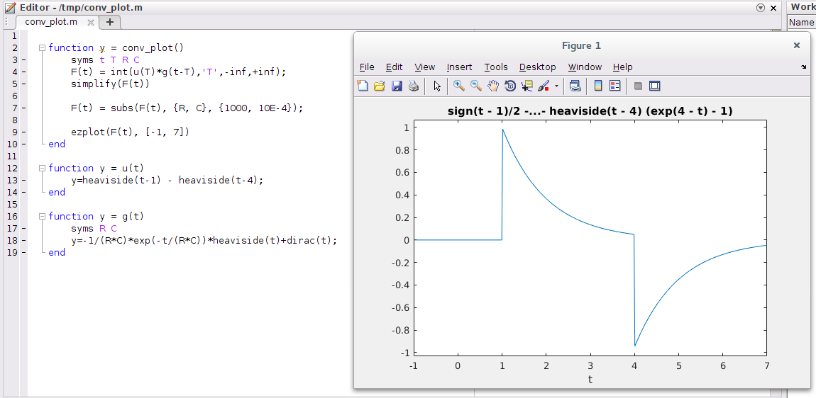
Matlab

Symbolic Math Toolbox needs to be installed for analytical calculations

function y = conv_plot()
    syms t T R C
    F(t) = int(u(T)*g(t-T),'T',-inf,+inf);
    simplify(F(t))
    
    F(t) = subs(F(t), {R, C}, {1000, 10E-4});
    
    ezplot(F(t), [-1, 7])
end

function y = u(t)
    y=heaviside(t-1) - heaviside(t-4);
end

function y = g(t)
    syms R C
    y=-1/(R*C)*exp(-t/(R*C))*heaviside(t)+dirac(t);
end

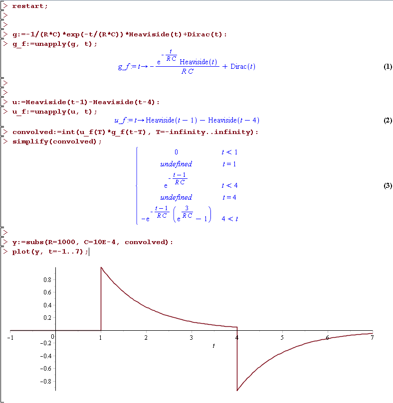
Maple

restart;

g:=-1/(R*C)*exp(-t/(R*C))*Heaviside(t)+Dirac(t):
g_f:=unapply(g, t);

u:=Heaviside(t-1)-Heaviside(t-4):
u_f:=unapply(u, t);

convolved:=int(u_f(T)*g_f(t-T), T=-infinity..infinity):
simplify(convolved);

y:=subs(R=1000, C=10E-4, convolved):
plot(y, t=-1..7);