NMPC with CasADi and Python – Part 2: Simulation of an uncontrolled system
CasADi is a powerful open-source tool for nonlinear optimization. It can be used with MATLAB/Octave, Python, or C++, with the bulk of the available resources referencing the former two options. This post series is intended to show a possible method of developing a simulation for an example system controlled by Nonlinear Model Predictive Control (NMPC) using CasADi and Python.
In this post, we will try to simulate an uncontrolled system with a forward Euler and a 4th order Runge-Kutta integration method. The latter can be the base for future closed-loop simulations.
As in the previous post, we will use a file ode.py to describe the system itself:
import casadi

def ode2(t, x, u):
    dx0 = casadi.tan(x[3]) * x[1] + 2*u[1] - 1
    dx1 = x[0] - casadi.sin(x[1])
    dx2 = 13 * x[3] + u[0] + 1
    dx3 = 0.2*x[0]

    return casadi.vertcat(dx0, dx1, dx2, dx3)
As we want to do numerical integration, we need to use some kind of integration method. For this, we could either use some library or implement one ourselves. As it’s not very complicated, we’ll do the latter. The integration methods will be defined in a file integration.py.
The simplest and first integration method we will implement is the Euler forward method. This method only uses a single evaluation of the derivative, i.e. it’s a first-order method:
 \approx \vec{x}(t) + \vec{\mathrm{ode}}(t,\vec{x},\vec{u}) h")
with 
def eulerforward(ode, h, t, x, u):
    xdot = ode(t, x, u)
    return x + xdot*h
We can test it and pass ode2 as argument with arbitrary state and control input values:
>>> from integration import eulerforward
>>> from ode import ode2
>>> eulerforward(ode2, 0.1, 0, [0,1,1,1], [1,1])
DM([0.255741, 0.915853, 2.5, 1])
Now let’s create a simulation.py file that actually simulates our system for multiple steps. We’ll use numpy for some convenience functions. Let’s define a few parameters:
import numpy as np
from integration import eulerforward
from ode import *

# parameters
t_0 = 0. # start time
t_end = 1. # end time
h = 0.01 # step size
t_arr = np.arange(t_0, t_end, h) # array of integration times
n_steps = len(t_arr) # number of steps
We define a control input that is static for the whole simulation and an initial state:
# states / control inputs
u_stat = np.array([0., 0.]) # static control input
x_0 = np.array([10, -5, 0.5, 1]) # initial state
We know define a data matrix that holds the values of x at all evaluated times as columns:
x = np.zeros([len(x_0), n_steps]) # holds states at different times as columns
x[:,0] = x_0 # set initial state for t_0
With the help of our integration function we can now evaluate the state for all time steps:
# simulate
for i in np.arange(1,n_steps): # skip 0th step
    x[:,i] = eulerforward(ode2, h, t_arr[i-1], x[:,i-1], u_stat).T
The .T after the function call transposes the array into a column vector so it fits into x.
Great! Now the simulation is done. But it would probably be nice to see a few graphs instead of only having numbers in a matrix – so let’s use matplotlib to show the states over time:
# plot results
from matplotlib import pyplot as plt

plt.plot(t_arr, x.T)

plt.legend(["x0", "x1", "x2", "x3"])
plt.xlabel("t")

plt.show()
All together:
import numpy as np
from integration import eulerforward
from ode import *

# parameters
t_0 = 0. # start time
t_end = 1. # end time
h = 0.01 # step size
t_arr = np.arange(t_0, t_end, h) # array of integration times
n_steps = len(t_arr) # number of steps

# states / control inputs
u_stat = np.array([0., 0.]) # static control input
x_0 = np.array([10, -5, 0.5, 1]) # initial state
x = np.zeros([len(x_0), n_steps]) # holds states at different times as columns
x[:,0] = x_0 # set initial state for t_0

# simulate
for i in np.arange(1,n_steps): # skip 0th step
    x[:,i] = eulerforward(ode2, h, t_arr[i-1], x[:,i-1], u_stat).T

# plot results
from matplotlib import pyplot as plt

plt.plot(t_arr, x.T)

plt.legend(["x0", "x1", "x2", "x3"])
plt.xlabel("t")

plt.show()
And you should see the following graph when you execute simulation.py:
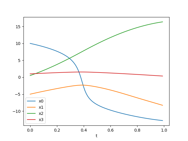
Not too shabby, right? Of course it’s only the behavior of an uncontrolled system, but a controller will get developed in later posts. First, let’s implement the second integration method: a Runge-Kutta 4th order integrator.
The Runge-Kutta 4th order method (RK4) uses four evaluations of the derivative and is used in many places. In general, a better approximation of the true integral can be expected than with methods of a lower order. The formulas can be found here. The implementation in integration.py can be done similar to the Euler forward method:
def rk4(ode, h, t, x, u):
    k1 = ode(t,x,u)
    k2 = ode(t+h/2, x+h/2*k1, u)
    k3 = ode(t+h/2, x+h/2*k2, u)
    k4 = ode(t+h,   x+h*k3, u)
    return x + h/6*(k1 + 2*k2 + 2*k3 + k4)
Let’s test it on the Python console:
>>> from integration import *
>>> from ode import *
>>> t = 0
>>> x = [1, 2, 3, 4]
>>> u = [0, 0]
>>> rk4(ode2, 0.01, t, x, u)
DM([1.01321, 2.00097, 3.53013, 4.00201])
>>> eulerforward(ode2, 0.01, t, x, u)
DM([1.01316, 2.00091, 3.53, 4.002])
So, the results seem to be similar but slightly different. Let’s replace eulerforward by rk4 in simulation.py and execute the script. Something like the following should appear:
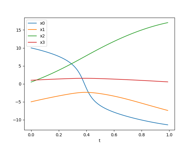
… which looks pretty much like before – at least to our eyes. Let’s evaluate the states with both eulerforward and rk4 and look at the difference to see how large it is! This is pretty straight forward, so here’s the resulting simulation.py and the graph of the difference over time:
import numpy as np
from integration import *
from ode import *

# parameters
t_0 = 0. # start time
t_end = 1. # end time
h = 0.01 # step size
t_arr = np.arange(t_0, t_end, h) # array of integration times
n_steps = len(t_arr) # number of steps

# states / control inputs
u_stat = np.array([0., 0.]) # static control input
x_0 = np.array([10, -5, 0.5, 1]) # initial state

# states with Euler integration
x_eul = np.zeros([len(x_0), n_steps]) # holds states at different times as columns
x_eul[:,0] = x_0 # set initial state for t_0

# states with RK4 integration
x_rk4 = np.zeros([len(x_0), n_steps])
x_rk4[:,0] = x_0

# simulate
for i in np.arange(1,n_steps): # skip 0th step
    # simulate with Euler
    x_eul[:,i] = eulerforward(ode2, h, t_arr[i-1], x_eul[:,i-1], u_stat).T
    # simulate with RK4
    x_rk4[:,i] = rk4(ode2, h, t_arr[i-1], x_eul[:,i-1], u_stat).T

# plot results
from matplotlib import pyplot as plt

# plot Euler results
plt.plot(t_arr, x_eul.T)
plt.title("States with Euler integration")
plt.legend(["x0", "x1", "x2", "x3"])
plt.xlabel("t")

# plot RK4 results
plt.figure() # new figure
plt.plot(t_arr, x_rk4.T)
plt.title("States with RK4 integration")
plt.legend(["x0", "x1", "x2", "x3"])
plt.xlabel("t")

# plot difference between Euler and RK4
plt.figure() # new figure
plt.plot(t_arr, (x_rk4 - x_eul).T)
plt.title("Difference between Euler and RK4 integration")
plt.legend(["x0", "x1", "x2", "x3"])
plt.xlabel("t")

plt.show()
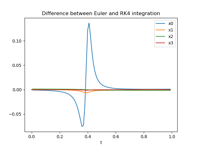
OK, we can see that the effect on one state is significantly larger than on the other states during this period of time. Whether the differences here are large or small depends on the system we simulated – as we haven’t based our example system on any real system we cannot really make a clear assessment here. Note that while the differences between the methods seem to get smaller towards the end, this is just a coincidence.
So, that’s it for today! In later posts we can have a look at actually controlling our simulated system.
Leave a Reply