NMPC with CasADi and Python – Part 3: State-space equations of a 2-DOF robot with SymPy or MATLAB

May 10, 2020 0 comments Article Uncategorized nspo

CasADi is a powerful open-source tool for nonlinear optimization. It can be used with MATLAB/Octave, Python, or C++, with the bulk of the available resources referencing the former two options. This post series is intended to show a possible method of developing a simulation for an example system controlled by Nonlinear Model Predictive Control (NMPC) using CasADi and Python.

In this post, we will look at determining the system equations of a robot with two degrees of freedom in stace-space form. These state-space equations can be used for simulation and for developing a nonlinear model predictive controller. For some transformation tasks, Python with SymPy will be utilized and an alternative using the MATLAB Symbolic Math Toolbox will be shown.

During the following, we are considering a robot with two links, two masses at the end of the links, and motors applying torque as control input at the joints. A diagram of the robot is shown below.

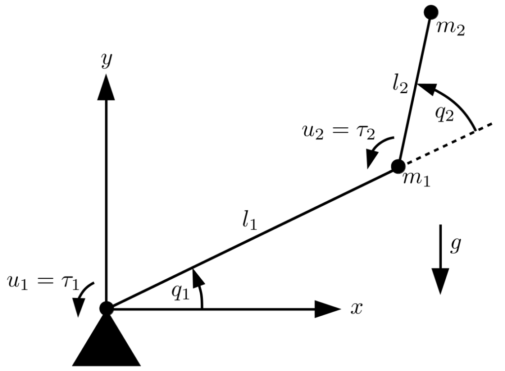
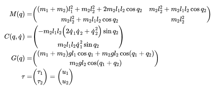
The set of nonlinear differential equations describing the dynamic behavior of a robot with joint angle vector $q = \begin{bmatrix} q_1 & q_2 & \ldots \end{bmatrix}^\intercal$ is often given in following form (or similarly; see e.g. Robot Modeling and Control by Spong et al.):

$M(q) \ddot{q} + C(q, \dot{q}) + G(q) = \tau$

In this equation, $M(q)$ is the mass or inertia matrix, $C$ is the coriolis matrix, and $G$ is the gravity vector. $\tau$ is the vector of control input torques applied at the joints.

Determining the relevant matrices of the equation above for the considered robot is possible through multiple methods. A commonly used one is applying the Lagrangian method. For this, the kinetic energy $T$ and the potential energy $V$ of the robot system must first be calculated using the generalized coordinates $q_j$ . The Lagrangian $L$ is then given by $L = T - V$ . The control input torque $\tau_j$ at each joint can be seen as a generalized force $Q_j$ . Now, one differential equation for each generalized coordinate $q_j$ can be found by using Lagrange’s equation of motion of the second kind:

$\frac{\mathrm{d}}{\mathrm{d}t}\frac{\partial L}{\partial \dot{q}_j} - \frac{\partial L}{\partial q_j} = Q_j$

For an equivalent robot system, the calculation steps are shown in Modeling of 2-DOF Robot Arm and Control by Okubanjo et al. Note, however, that there are some inaccuracies in this paper: Equation 13 is incorrect due to two missing squared operators. This is corrected from equation 15 onwards. Furthermore, the matrix form of the differential equation shown in equation 38 contains an additional $\dot{\theta}$ after the coriolis matrix. While this is generally not incorrect and an alternative form of the convention, the results in equation 34 and 35 do not fit to this form. Due to these problems, using the results from this paper cannot be recommended without double-checking. Bingül et al. (A Fuzzy Logic Controller tuned with PSO for 2 DOF robot trajectory control) considered the same robot configuration though, and with their results the calculations should lead to the following matrices and vectors (for the aforementioned matrix formulation of the robot system equation):

These equations cannot be fed directly into CasADi though – we need a state-space representation. An obvious choice of a state vector for this system would be the two joint angles and angular velocities ( $x = \begin{bmatrix} q_1 & \dot{q_1} & q_2 & \dot{q_2} \end{bmatrix}^\intercal$ ). Due to the relation of a joint angle and its angular velocity, two rows of the system equation will simply be

$\frac{\mathrm{d}}{\mathrm{d}t} q_1 = \dot{q_1}\\ \frac{\mathrm{d}}{\mathrm{d}t} q_2 = \dot{q_2}$

The other two rows for $\frac{\mathrm{d}}{\mathrm{d}t} \dot{q_1}$ and $\frac{\mathrm{d}}{\mathrm{d}t} \dot{q_2}$ can be calculated from the set of nonlinear differential equations above. This transformation can either be done by hand, or by using a tool like SymPy or the MATLAB Symbolic Math Toolbox. For this, all symbolic variables must first be defined, then the equations need to be defined, and finally it is possible to tell the tool to solve for the variables of interest.

Code for Python / SymPy:

#!/usr/bin/env python3

from sympy import *

# masses of robot arms
m1, m2 = symbols("m1 m2")

# lengths of robot arms
l1, l2 = symbols("l1 l2")

# acceleration due to gravity
g = symbols("g")

# angles at robot joints
q1, q2 = symbols("q1 q2")

# 1st derivatives of angles
dq1, dq2 = symbols("dq1 dq2")

# 2nd derivatives of angles
ddq1, ddq2 = symbols("ddq1 ddq2")
ddq = Matrix([ddq1,
              ddq2])

# control input torque
u1, u2 = symbols("u1 u2")
U = Matrix([u1, u2])

# matrix coefficients for intertia matrix M(q)
M11 = (m1+m2)*l1**2 + m2*l2**2 + 2*m2*l1*l2*cos(q2)
M12 = m2*l2**2 + m2*l1*l2*cos(q2)
M21 = m2*l2**2 + m2*l1*l2*cos(q2)
M22 = m2*l2**2
M = Matrix([[M11, M12], [M21, M22]])

# matrix coefficients for coriolis matrix C(q, dq)
C11 = -m2*l1*l2*(2*dq1*dq2 + dq2**2)*sin(q2)
C21 = m2*l1*l2*dq1**2*sin(q2)
C = Matrix([C11, C21])

# matrix coefficients for gravity vector G(q)
G11 = (m1 + m2)*g*l1*cos(q1) + m2*g*l2*cos(q1+q2)
G21 = m2*g*l2*cos(q1+q2)
G = Matrix([G11, G21])

# dynamic equations of robot
eq = Eq(U, M*ddq + C + G)

sol = solve(eq, (ddq1, ddq2))

print("ddq1 = {} \n\nddq2 = {}".format(sol[ddq1], sol[ddq2]))

This yields the missing two lines of the state-space system equation:

> python3 transform_equations_2dof.py 
ddq1 = (l2*(2*dq1*dq2*l1*l2*m2*sin(q2) + dq2**2*l1*l2*m2*sin(q2) - g*l1*m1*cos(q1) - g*l1*m2*cos(q1) - g*l2*m2*cos(q1 + q2) + u1) + (l1*cos(q2) + l2)*(dq1**2*l1*l2*m2*sin(q2) + g*l2*m2*cos(q1 + q2) - u2))/(l1**2*l2*(m1 + m2*sin(q2)**2)) 

ddq2 = -(l2*m2*(l1*cos(q2) + l2)*(2*dq1*dq2*l1*l2*m2*sin(q2) + dq2**2*l1*l2*m2*sin(q2) - g*l1*m1*cos(q1) - g*l1*m2*cos(q1) - g*l2*m2*cos(q1 + q2) + u1) + (dq1**2*l1*l2*m2*sin(q2) + g*l2*m2*cos(q1 + q2) - u2)*(l1**2*m1 + l1**2*m2 + 2*l1*l2*m2*cos(q2) + l2**2*m2))/(l1**2*l2**2*m2*(m1 + m2*sin(q2)**2))

Code for MATLAB / Symbolic Math Toolbox (this script can also be run with Octave, which then uses SymPy in the background):

% masses of robot arms
syms m1 m2;

% lengths of robot arms
syms l1 l2;

% acceleration due to gravity
syms g;

% angles at robot joints
syms q1 q2;

% 1st derivatives of angles
syms dq1 dq2;

% 2nd derivatives of angles
syms ddq1 ddq2;
ddq = [ddq1; ddq2];

% control input torque
syms u1 u2;
U = [u1; u2];

% matrix coefficients for inertia matrix M(q)
M11 = (m1+m2)*l1^2 + m2*l2^2 + 2*m2*l1*l2*cos(q2);
M12 = m2*l2^2 + m2*l1*l2*cos(q2);
M21 = m2*l2^2 + m2*l1*l2*cos(q2);
M22 = m2*l2^2;
M = [M11, M12; M21, M22];

% matrix coefficients for coriolis matrix C(q, dq)
C11 = -m2*l1*l2*(2*dq1*dq2 + dq2^2)*sin(q2);
C21 = m2*l1*l2*dq1^2*sin(q2);
C = [C11; C21];

% matrix coefficients for gravity vector G(q)
G11 = (m1 + m2)*g*l1*cos(q1) + m2*g*l2*cos(q1+q2);
G21 = m2*g*l2*cos(q1+q2);
G = [G11; G21];

% dynamic equations of robot
eq = M*ddq + C + G == U;

sol = solve(eq, [ddq1, ddq2]);

disp(ddq1 == sol.ddq1);
disp('');
disp(ddq2 == sol.ddq2);

NMPC with CasADi and Python – Part 3: State-space equations of a 2-DOF robot with SymPy or MATLAB

Leave a Reply Cancel reply

Recent Posts

Recent Comments

Archives

Categories

Meta